1. Introduction to Programming Concepts
"In reality, programming languages are how programmers express and communicate ideas - and the audience for those ideas is other programmers, not computers. The reason: the computer can take care of itself, but programmers are always working with other programmers, and poorly communicated ideas can cause expensive flops."
- Guido van Rossum, creator of Python
- In this chapter, you will get introduced to the most important concepts in programming.
- Later chapters will give a deeper understanding of these concepts (and add other concepts).
Table of contents
- 1. Calculator
- 2. Variables
- 3. Functions
- 4. Lists
- 5. Functions over Lists
- 6. Complexity
- 7. Lazy Evaluation
- 8. Higher-Order Programming
- 9. State
- 10. Objects and Classes
- 11. Concurrency
- 12. Concurrency with State
- 13. Chapter Summary
1. Calculator
One of the simplest and most immediate things a programming environment can do is perform calculations. This is a great way to verify your setup and get a feel for the language's syntax.
- In Python, the interactive interpreter (also called a REPL: Read-Eval-Print Loop) is the perfect tool for this. Start it by typing
python3orpythonin your terminal. You'll see a>>>prompt. - At the prompt, type:
>>> 9999 * 9999 - Result:
99980001 - Info:
- The Python interpreter reads your line of code, evaluates the expression, and prints the result.
- This immediate feedback loop is a powerful tool for learning and experimenting.
- In a script file (e.g.,
myscript.py), you would use theprint()function to display output:print(9999 * 9999).
2. Variables
Variables are names used to store and refer to values. Using variables allows us to break down complex calculations into simpler steps and reuse results.
Conceptual Model: Single-Assignment Variables (Oz)
In some programming models, a variable is like a mathematical constant: once you give it a value, it never changes. This is known as single assignment or immutable binding.
- The Oz language enforces this. The
declarestatement creates a new variable and binds it to a value.declare V = 9999 * 9999 {Browse V*V} - Info:
- In this model, variables are short-cuts for values, they cannot be assigned more than once. This can prevent certain types of bugs where a variable is changed unexpectedly.
Python Implementation: Mutable Variables
In Python (and most mainstream languages), variables are mutable. A variable name is a label that points to a value, and you can move that label to point to a different value at any time.
- Declare and use a variable in Python:
v = 9999 * 9999 print(v * v) - Result:
9996000599960001 - Info:
- Python variables are created with a simple assignment (
=). - Unlike the Oz model, you can re-assign a Python variable to a new value:
v = 100 # v now points to 100 v = "hello" # It can even point to a different type - By convention, programmers use
UPPERCASE_SNAKE_CASEfor variables they intend to be constants, even though the language doesn't enforce it:MY_CONSTANT = 9999.
- Python variables are created with a simple assignment (
Thought Experiment: The Limits of Variables
Now, consider the problem of calculating 100 factorial (written as 100!), which is the product of all positive integers up to 100 (1 * 2 * 3 * ... * 100).
With only the concepts we've introduced so far (calculation and variables), could you write a program for this without manually typing out all 100 numbers? This need for repetition and abstraction leads us directly to our next, and most powerful, concept: functions.
3. Functions
Functions are the primary tool for creating abstractions in programming. They allow us to package a computation, give it a name, and reuse it with different inputs (arguments). This solves the problem of repetition we identified in the previous section.
Factorial
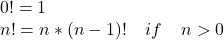
The factorial of a non-negative integer n, denoted n!, is the product of all positive integers less than or equal to n. Its formal definition is recursive:
- Factorial of 10:
1*2*3*4*5*6*7*8*9*10results in3628800. - We can implement this definition directly using a function that calls itself. This is called recursion.
Conceptual Model: Recursive Definition (Oz)
-
The Oz implementation mirrors the mathematical definition closely using an
if/elseexpression.declare fun {Fact N} if N==0 then 1 else N*{Fact N-1} end end
Python Implementation
-
Python's syntax is very similar. We use the
defkeyword to define a function andreturnto specify its output.def fact(n): if n == 0: return 1 else: return n * fact(n - 1) -
Calling the function:
print(fact(10)) -
Result:
3628800 -
Python has built-in support for arbitrarily large integers, so we can easily compute
fact(100):print(fact(100)) -
Result:
93326215443944152681699238856266700490715968264381621468592963895217599993229915608941463976156518286253697920827223758251185210916864000000000000000000000000
In Python's World: Recursion Depth Limits
While recursion is a powerful conceptual tool, Python (like many practical languages) has a recursion depth limit (usually around 1000 calls) to prevent a type of error called a "stack overflow." If you tried to call fact(3000), it would fail with an error.
For problems that require very deep recursion, a Python programmer would typically rewrite the function using a simple loop (an iterative approach). This is a common trade-off: conceptual elegance (recursion) vs. practical constraints (memory).
Checkpoint
In the recursive `fact(n)` function, what is the base case and what is the recursive step?
- Base Case:
if n == 0: return 1. This is the condition that stops the recursion. - Recursive Step:
return n * fact(n - 1). This is where the function calls itself with a smaller version of the problem.
Exercise: The Fibonacci Sequence
The Fibonacci sequence is another famous mathematical sequence defined recursively: F(n) = F(n-1) + F(n-2), with the base cases F(0) = 0 and F(1) = 1.
- Write a Python function
fib(n)that calculates the nth Fibonacci number.
Hint
You will need two base cases in your if/elif/else structure.
Food for thought: Try running fib(40). You'll notice it's surprisingly slow. This is because, like our slow_pascal example later, it recalculates the same values over and over. We will fix this performance problem in the "Complexity" section.
Combinations
We can build more complex functions by composing simpler ones. This is known as functional abstraction. For example, the "combination" formula, which calculates how many ways you can choose r items from a set of n items, is defined using factorials:

Oz Definition
declare
fun {Comb N R}
    {Fact N} div ({Fact R}*{Fact N-R})
end
Python Implementation
-
We can define a
combfunction that calls our existingfactfunction. -
Note: The result of a combination is always an integer, so we use integer division (
//in Python) instead of floating-point division (/).def comb(n, r): return fact(n) // (fact(r) * fact(n - r)) -
Calling the function:
print(comb(10, 3)) -
Result:
120
Exercise: Permutations
The formula for permutations, which calculates the number of ways to order r items from a set of n, is P(n, r) = n! / (n-r)!.
- Using functional abstraction, write a Python function
perm(n, r)that uses your existingfactfunction to calculate permutations.
4. Lists
A list is an ordered sequence of elements. In Python, lists are a versatile, built-in data type that can hold elements of any type.
- A list literal is created with square brackets:
my_list = [5, 6, 7, 8]
print(my_list)
The Head and Tail Model
While Python's lists are technically implemented as dynamic arrays, it is extremely useful for many algorithms to think of them recursively, as a pair of two things:
- Head: The first element of the list.
- Tail: A list containing all the other elements.
This "Head/Tail" structure is the fundamental building block of lists in many functional programming languages.
Conceptual Model: The "Cons" Cell (Oz)
- In Oz (and languages like Lisp), a list is explicitly a chain of links. Each link, often called a cons cell, contains two things: a value (the head) and a reference to the rest of the chain (the tail). The chain ends with a special
nilvalue. [6 7]is represented as6 -> 7 -> nil.- The
H|Tsyntax (pronounced "H-bar-T") is used to construct a list from a headHand a tailT.declare H = 5 T = [6 7 8] {Browse H|T} - Result:
[5 6 7 8]
Deconstructing and Reconstructing Lists in Python
To work with lists recursively, we need ways to get their constituent parts (like the head and tail) and put them back together.
Using Indexing and Slicing
- The most common way to deconstruct a list is to use indexing for single elements and slicing for sub-lists.
L = [5, 6, 7, 8] head = L[0] tail = L[1:] # A slice from index 1 to the end print(f"Head: {head}") print(f"Tail: {tail}") - The simplest way to reconstruct a list is with list concatenation (
+):new_list = [head] + tail print(new_list) # Output: [5, 6, 7, 8]
Pattern Matching
Manually checking list length and slicing can be clumsy. A more elegant and powerful technique is pattern matching, which lets us declaratively deconstruct a data structure.
Conceptual Model: case in Oz
- Oz uses the
casestatement to match a list against theH|Tpattern, automatically binding the head toHand the tail toT.declare L = [5 6 7 8] case L of H|T then {Browse H} {Browse T} end - Result:
5and[6 7 8]
Python Implementation: match statement
-
As of Python 3.10, Python has a powerful
matchstatement that brings this declarative style directly into the language. -
We can match a list against various patterns. The
*syntax is used to capture multiple items into a new list.L = [5, 6, 7, 8] match L: case []: # Matches an empty list print("The list is empty.") case [element]: # Matches a list with exactly one element print(f"The list has one element: {element}") case [head, *tail]: # Matches a list with at least one element print(f"Head: {head}") print(f"Tail: {tail}") -
Info:
- The
matchstatement is the recommended way to deconstruct data structures in modern Python. It is less error-prone and more readable than manual indexing and slicing. - Before Python 3.10, a similar effect could be achieved with "extended unpacking":
head, *tail = L, but this required a separate check for the empty list case.
- The
Exercise: Swap First and Last
- Write a Python function
swap_first_last(a_list)that takes a list and returns a new list where the first and last elements have been swapped. - Handle the edge cases: what should happen if the list is empty or has only one element? (It should return the list unchanged).
Hint
For a list with two or more elements, you can deconstruct it into three parts: the first element, the middle elements, and the last element. Then, reconstruct it in a new order. The match [first, *middle, last]: pattern is perfect for this.
5. Functions over Lists
Now that we have functions and a way to think about lists recursively (as a head and a tail), we can write functions that process lists. The structure of these functions will often mirror the recursive structure of the list itself.
A typical recursive function over a list has two main parts:
- Base Case: What to do when the list is empty (or has some other simple form). This stops the recursion.
- Recursive Step: How to process the head of the list, and then call the function again on the tail of the list.
Example: Pascal's Triangle
Pascal's triangle is a famous number pattern where each number is the sum of the two numbers directly above it.
      1
     1 1
    1 2 1
   1 3 3 1
  1 4 6 4 1
We can define a function, pascal(n), which calculates the nth row of the triangle. The key insight is that we can calculate any row from the row above it. For example, to get the fifth row ([1 4 6 4 1]) from the fourth ([1 3 3 1]):
- Pad the fourth row with a zero on the left and right.
[1 3 3 1 0](Shifted left)[0 1 3 3 1](Shifted right)
- Sum the two padded lists element by element.
[1+0, 3+1, 3+3, 1+3, 0+1] = [1 4 6 4 1]
This gives us a clear algorithm that we can implement with several helper functions.
Python Implementation
This problem is a great example of top-down design: we'll write the main pascal function first, assuming our helper functions exist, and then we'll implement the helpers.
def pascal(n):
    """Calculates the nth row of Pascal's triangle (1-indexed)."""
    # Base Case
    if n == 1:
        return [1]
    # Recursive Step
    else:
        previous_row = pascal(n - 1)
        # Assumes helper functions exist
        shifted_left = shift_left(previous_row)
        shifted_right = shift_right(previous_row)
        return add_lists(shifted_left, shifted_right)

def shift_left(a_list):
    """Pads a list with a 0 on the right."""
    return a_list + [0]

def shift_right(a_list):
    """Pads a list with a 0 on the left."""
    return [0] + a_list

def add_lists(list1, list2):
    """Adds two lists element-wise."""
    # We can use a list comprehension with zip to do this concisely
    return [x + y for x, y in zip(list1, list2)]

# Execute and see the result
print(pascal(5))
# Result: [1, 4, 6, 4, 1]

print(pascal(20))
# Result: [1, 19, 171, 969, 3876, 11628, 27132, 50388, 75582, 92378, 92378, 75582, 50388, 27132, 11628, 3876, 969, 171, 19, 1]
Python Toolbox:
zipand List Comprehensions
zip(list1, list2)is a built-in function that takes two (or more) lists and "zips" them into a sequence of pairs (tuples). For example,zip([1, 2], [3, 4])produces(1, 3)and then(2, 4).[... for ... in ...]is a list comprehension. It's a concise and "Pythonic" way to create a new list. The expression[x + y for x, y in zip(list1, list2)]reads like English: "Create a new list containingx + yfor each pairx, yyou get from zipping the two lists."
Exercise: Recursive List Sum
- Write a recursive function
sum_list(numbers)that takes a list of numbers and returns their sum. - Follow the recursive pattern:
- Base Case: The sum of an empty list is 0.
- Recursive Step: The sum of a non-empty list is its
headplus the sum of itstail.
- Use a
matchstatement (or slicing) to deconstruct the list.
6. Complexity
The implementation of pascal we wrote in the previous section is actually quite efficient. We were careful to compute the recursive step pascal(n - 1) only once and store its result in the previous_row variable.
To understand a critical concept in performance, let's explore what happens if we aren't so careful. Consider a slightly different, more direct implementation that reveals a common and serious pitfall with recursion. The field of computer science that studies the performance of algorithms is called complexity analysis.
The Problem: Redundant Computations
Let's write a naive version of the function, slow_pascal, where we call the function directly inside our add_lists call, instead of storing the intermediate result.
# A deliberately inefficient version to demonstrate the complexity issue
def slow_pascal(n):
    if n == 1:
        return [1]
    else:
        # We call slow_pascal(n-1) TWICE, once for each helper.
        return add_lists(
            shift_left(slow_pascal(n - 1)),
            shift_right(slow_pascal(n - 1))
        )
If you try running slow_pascal(30), you will notice it takes a surprisingly long time to complete.
-
Why is this slow?
Answer
Calling
slow_pascal(n)results in two separate calls toslow_pascal(n-1). Each of those calls results in two calls toslow_pascal(n-2), and so on. The number of calls grows exponentially.A single call to
slow_pascal(30)will end up callingslow_pascal(1)over 500 million times (229 times, to be exact).
The Solution: Store and Reuse
The solution is simple: we must avoid re-computing slow_pascal(n-1). We can do this by calling it just once, storing its result in a local variable, and then reusing that variable.
This is, in fact, the version we wrote in the previous section. Let's rename it to fast_pascal for clarity.
def fast_pascal(n):
    if n == 1:
        return [1]
    else:
        # Call the function just ONCE and store the result.
        previous_row = fast_pascal(n - 1)
        return add_lists(
            shift_left(previous_row),
            shift_right(previous_row)
        )
- Info:
- By introducing the
previous_rowvariable, we ensure the recursive call for eachnhappens only once. - This small change has a massive impact on performance.
- By introducing the
Time Complexity
Time complexity is a way to describe how the runtime of an algorithm grows as the size of the input grows.
-
What is the time complexity of
slow_pascal(n)andfast_pascal(n)?Answer
slow_pascal(n): The number of calls roughly doubles for each increment ofn. This is exponential time, often written as O(2n).fast_pascal(n): The function is calledntimes. In each call, we do work proportional to the length of the row, which is alson. This is polynomial time, roughly O(n2).
Exponential time algorithms are generally considered impractical for anything but small inputs.
Exercise 1: See the Difference
- Use Python's built-in
timemodule to measure and compare the execution time ofslow_pascal(n)andfast_pascal(n)forn=20,n=21,n=22. What do you observe?
import time

# Example usage of the time module
start_time = time.time()
result = fast_pascal(20) # or slow_pascal(20)
end_time = time.time()

print(f"Calculation took {end_time - start_time:.4f} seconds.")
Exercise 2: Memoizing Fibonacci
The recursive fib(n) function you wrote in a previous section suffers from exponential time complexity. You can see this if you try to run fib(40).
- Create a more efficient version called
fast_fib(n). - A common technique for this is memoization: using a dictionary (or "cache") to store results that have already been computed.
Hint
Create a dictionary memo = {} that is accessible to your function. Inside the function, before you compute fib(n), first check if n is already a key in memo. If it is, return the stored value immediately. If not, compute the result, store it in memo before you return it, and then return it.
The Pythonic Way: functools.lru_cache
This problem is so common that Python has a built-in tool for it called a decorator. The @lru_cache decorator automatically adds memoization to any function you place it on top of. This is the preferred way to solve this in modern Python.
from functools import lru_cache

@lru_cache(maxsize=None) # The decorator that does all the work.
def fib_pythonic(n):
    if n <= 1:
        return n
    return fib_pythonic(n - 1) + fib_pythonic(n - 2)

# This version is also instantaneous and requires no manual cache management.
print(fib_pythonic(100))
7. Lazy Evaluation
Up until now, every function call we've made has been executed immediately. When we call fast_pascal(30), the entire computation for all 30 rows happens before the result is returned. This is known as eager evaluation.
An alternative strategy is lazy evaluation: a calculation is deferred and only performed when its result is actually needed. This allows us to work with concepts like potentially infinite data structures without running out of memory or getting stuck in an infinite loop.
In Python, the primary tool for lazy evaluation is the generator.
Generators and the yield Keyword
A generator is a special kind of function that, instead of returning a single value, can yield a sequence of values one at a time. When a generator function is called, it doesn't run. It returns a generator object, which is an iterator that knows how to produce the values on demand.
- An example generator that can produce a list of integers from
Nto infinity:def lazy_ints_from(n): """A generator that yields integers starting from n, forever.""" current = n while True: yield current current += 1 - Info:
- The
yieldstatement pauses the function's execution and sends a value back to the caller. When the caller asks for the next value, the function resumes right where it left off. - If we call
lazy_ints_from(0), it immediately returns a generator object. No code inside thewhileloop runs yet.>>> numbers = lazy_ints_from(0) >>> print(numbers) <generator object lazy_ints_from at 0x...> - The computation only happens when we ask for a value using the built-in
next()function.>>> next(numbers) 0 >>> next(numbers) 1 >>> next(numbers) 2 - Because the values are generated on demand, we can represent an infinite sequence without running out of memory.
- The
Checkpoint
-
In the
lazy_ints_fromgenerator, what would happen if you replacedyield currentwithreturn current?Answer
The function would no longer be a generator. It would execute the loop once,
returnthe initial value ofcurrent(n), and then terminate completely. It could not produce a sequence of values.
Exercise 1
-
What happens if you try to call
sum(lazy_ints_from(0))? Is this a good idea? Why or why not?Hint
The recursive
sum_listneeds to reach the end of the list to find its base case. Does an infinite list have an end?
Lazy Calculation of Pascal's Triangle
We can use a generator to produce the rows of Pascal's triangle one by one, infinitely. This is a very powerful pattern: the producer (pascal_rows_generator) only calculates the next row when the consumer asks for it.
def pascal_rows_generator():
    """A generator that yields the rows of Pascal's triangle, forever."""
    current_row = [1]
    while True:
        yield current_row
        # Calculate the next row based on the current one
        current_row = add_lists(
            shift_left(current_row),
            shift_right(current_row)
        )

# Example Usage
pascal_gen = pascal_rows_generator()

# We can pull as many rows as we need
print(next(pascal_gen))  # Output: [1]
print(next(pascal_gen))  # Output: [1, 1]
print(next(pascal_gen))  # Output: [1, 2, 1]

# We can also use it in a for loop with a condition to stop
print("The first 10 rows:")
ten_rows = []
for i, row in enumerate(pascal_gen):
    ten_rows.append(row)
    if i == 9: # We need to stop it manually
        break
print(ten_rows)
Exercise 2
-
The lazy version is often more efficient than an eager version that calculates N rows at once.
-
Imagine you have a function
get_n_pascal_rows(n)that eagerly calculates and returns a list of the firstnrows. -
Think of a scenario where you first need 10 rows, and then later you need the 11th row. Why is the generator version (
pascal_rows_generator) more optimal in this situation?Hint
When you call
get_n_pascal_rows(10)and thenget_n_pascal_rows(11), how many rows are being recalculated? What about the generator version?Answer
The eager function
get_n_pascal_rows(11)would have to recalculate the first 10 rows from scratch. The generator, however, maintains its state. It already has the 10th row computed and can generate the 11th row in a single, efficient step.
Exercise 3: Recursive Generator
Generators can also be written recursively. A recursive generator is a function that typically does two things:
- It
yields one or more values based on its current state. - It uses
yield fromto delegate to a recursive call with a new state.
A key technique used in this style of recursion is the accumulator. An accumulator is an argument to a function that carries the state of the computation forward into the next recursive call. In this exercise, the current_row parameter will act as our accumulator. We will explore accumulator-based patterns in more detail in a later chapter.
- Write a recursive generator function
pascal_rows_generator_recursive(current_row). You can give the parameter a default value of[1]to make the initial call easier. - The function should:
- Take the current row as an argument (the accumulator).
- Inside the function, you should:
yieldthecurrent_row.- Calculate the
next_row. yield froma recursive call topascal_rows_generator_recursivewith thenext_row.
Hint
The yield from <expression> statement allows one generator to delegate part of its operations to another generator. In this case, you are delegating to a recursive call of the same generator. The structure will be very concise.
8. Higher-Order Programming
So far, we have treated functions as recipes for computation. Higher-order programming introduces a powerful new perspective: it treats functions themselves as values, just like numbers, strings, or lists.
A language supports higher-order programming if its functions are first-class citizens. This means you can:
- Assign a function to a variable.
- Pass a function as an argument to another function.
- Return a function from another function.
This capability allows us to write more abstract and reusable code. Let's look at the two most important techniques this enables.
1. Passing Functions as Arguments (Genericity)
The most common use of higher-order programming is to write generic functions that can be customized by passing in other functions as arguments.
Imagine we want to apply an operation to every number in a list. Instead of writing a separate function for squaring, another for cubing, and another for adding one, we can write a single, generic function.
def apply_to_list(numbers, operation_func):
    """Applies a function to every number in a list."""
    result = []
    for number in numbers:
        # Call the function that was passed in
        result.append(operation_func(number))
    return result

# --- Define some simple operations ---
def square(n):
    return n * n

def add_one(n):
    return n + 1

# --- Use our generic function ---
my_numbers = [1, 2, 3, 4]

squared = apply_to_list(my_numbers, square)
print(f"Squared: {squared}") # Output: Squared: [1, 4, 9, 16]

incremented = apply_to_list(my_numbers, add_one)
print(f"Incremented: {incremented}") # Output: Incremented: [2, 3, 4, 5]
By passing in different functions (square, add_one), we completely changed the behavior of apply_to_list without modifying its code.
Python Toolbox:
lambdafor Anonymous FunctionsSometimes you need a simple function for just one use and don't want to give it a full
defname. Python'slambdakeyword lets you create small, anonymous functions on the fly.The syntax is
lambda arguments: expression.# Using our generic function with a lambda my_numbers = [1, 2, 3, 4] cubed = apply_to_list(my_numbers, lambda n: n ** 3) print(f"Cubed: {cubed}") # Output: Cubed: [1, 8, 27, 64]
2. Returning Functions from Functions (Instantiation)
Just as you can pass a function in, you can also return a function as a result. This allows you to create "function factories" - functions that generate and configure other functions.
When a function is created inside another function, it forms a closure. A closure is a function that "remembers" the variables from the environment where it was created, even after the outer function has finished.
def make_multiplier(n):
    """A factory that makes functions that multiply by n."""
    def multiplier(x):
        # This inner function "remembers" the value of n
        return x * n
    return multiplier # We return the function object itself

# Create a function that multiplies by 5
times_5 = make_multiplier(5)

# Create another function that multiplies by 10
times_10 = make_multiplier(10)

# The generated functions work as expected
print(times_5(4))  # Output: 20 (it remembers n=5)
print(times_10(4)) # Output: 40 (it remembers n=10)
Here, times_5 is a closure. It holds onto the n=5 from its creation, and times_10 holds onto n=10. This is a powerful way to create specialized functions from a general template.
We have only scratched the surface. These fundamental ideas (passing and returning functions) are the building blocks for many advanced programming patterns. In a later chapter on Declarative Programming, we will build on this foundation to explore Python's powerful built-in tools like map and filter, and advanced concepts like decorators.
Exercise: Greeter Factory
- Write a function factory
create_greeter(greeting)that returns a new function. - The function it returns should take one argument,
name, and return a string likef"{greeting}, {name}!". - Use it to create a
say_hellofunction and asay_goodbyefunction and test them.
9. State
All the functions we have written so far share a common property: if you call them with the same inputs, they will always produce the same output. A function like add(2, 3) will always return 5. This style of programming is called stateless or declarative. It's predictable and easy to reason about.
However, sometimes we need components that can change over time. We need them to remember things from past events. This "memory" is called explicit state. A component with state can produce different results for the same call, depending on its history.
Conceptual Model: The Memory Cell (Oz)
To support explicit state, the declarative model needs to be extended with a new concept: a container for a value that can be changed. In Oz, this is called a cell.
A cell has three basic operations:
{NewCell 0}: Create a new cell with an initial value of0.@C: Read the current value of cellC.C := ...: Assign a new value to cellC.
Using a cell, we can create a function that "remembers" how many times it has been called.
- An Oz function with memory:
declare C = {NewCell 0} fun {Add A B} C := @C + 1 A + B end - Info:
- The cell
Cis created once, outside the function. It acts as a long-term memory. - Each time
Addis called, it reads the value fromC, adds one to it, and writes the new value back into the cell. The cell's state persists between calls.
- The cell
Python Implementation: Mutable State
In Python, we don't need a special "cell" concept because variables can already point to mutable objects (like lists or dictionaries), and variables in a wider scope can be modified. Explicit state is about managing data that lives longer than a single function call.
The simplest way to implement the counter is with a global variable.
# A global variable to hold the state
call_count = 0

def add_with_counter(a, b):
    # 'global' keyword is needed to modify the variable
    global call_count
    call_count = call_count + 1
    return a + b

print(f"Result: {add_with_counter(2, 3)}, Count: {call_count}")
print(f"Result: {add_with_counter(10, 20)}, Count: {call_count}")
- Result:
Result: 5, Count: 1 Result: 30, Count: 2 - Info:
- The
call_countvariable exists outside the function and holds its value across multiple calls. - We must use the
globalkeyword to tell Python we intend to modify the global variable, not create a new local one.
- The
A Better Way: Encapsulation
Using global variables is simple, but it can be risky in larger programs. Any part of the program can modify call_count, which can lead to bugs that are hard to track down.
A much better approach is to encapsulate the state so it is not exposed globally. We can bundle the state and the functions that operate on it together into a single unit. This idea is the foundation of object-oriented programming and leads directly to our next section: objects and classes.
Exercise: A Simple Accumulator
- An accumulator is a stateful component that adds every input it receives to a running total.
- Create a function
accumulate(n)that uses a global variabletotal(initialized to 0). - Each call to
accumulate(n)should addntototaland return the new total. - Example calls:
print(accumulate(5))   # Should print 5
print(accumulate(10))  # Should print 15
print(accumulate(3))   # Should print 18
10. Objects and Classes
In the last section, we saw that global variables can create state, but they are fragile. Any part of a program can change them. Object-Oriented Programming (OOP) offers a powerful solution to this problem: encapsulation.
The idea is to create "objects," which are self-contained units that bundle together:
- State: The data or "memory" the object holds.
- Behavior: The functions (called methods) that can operate on that state.
By encapsulating state inside an object, we can protect it from accidental modification and create clear, reusable components.
Conceptual Model: A Function Factory (Oz)
In Oz, you can create an object by defining a function that acts as a "factory." This factory function creates a local, hidden memory cell and then returns a package of other functions (a record) that are the only ones allowed to access that cell.
- The
NewCounterfactory in Oz:declare fun {NewCounter} C = {NewCell 0} // Create a hidden, local state fun {Bump} ... end // Define inner functions that fun {Read} ... end // can access that state in counter(bump:Bump read:Read) // Return the functions end - Info:
- Each time
{NewCounter}is called, it creates a new, independent cellC. - The
BumpandReadfunctions it creates inside are closures - they "remember" the specificCthey were created with. - The factory returns a record containing these functions. The cell
Cis completely hidden from the outside world. - This allows for multiple, independent counter objects:
Ctr1 = {NewCounter}
Ctr2 = {NewCounter}
{Ctr1.bump} // Ctr1's cell is now 1
{Ctr2.read} // Ctr2's cell is still 0
- Each time
Exercise: Recreating the Factory in Python
Before we learn Python's dedicated syntax for objects, let's replicate the Oz factory pattern directly. This will help you understand the core concept of a closure.
- Write a Python function
make_counter(). - Inside
make_counter, create a local variablecountinitialized to0. - Define two inner functions,
bump()andread().bump()should increment thecountvariable and return its new value.read()should just return the current value ofcount.
make_countershould return the two inner functions. A good way to do this is to return them in a dictionary, like{"bump": bump, "read": read}.- Test your factory by creating two separate counters and verifying that their states are independent.
Hint
When an inner function needs to modify a variable from its containing function's scope (not a global variable), you need to use the nonlocal keyword. For example: nonlocal count. You won't need it for the read function.
The Pythonic Way: The class Keyword
While the function factory pattern is powerful, Python provides a more direct and conventional syntax for creating object blueprints: the class. A class is a formal blueprint for creating objects, and it's the standard for object-oriented programming in Python.
Let's rewrite our counter using this much cleaner approach.
class Counter:
    """A blueprint for creating counter objects."""

    # The __init__ method is the constructor.
    # It runs when a new object is created.
    def __init__(self):
        # The state is stored on the instance ('self').
        # The underscore prefix `_count` is a convention
        # to indicate it's for internal use.
        self._count = 0

    # A method to change the state
    def bump(self):
        self._count += 1
        return self._count

    # A method to read the state
    def read(self):
        return self._count

# --- Creating and using instances of the class ---
# Instantiation: calling the class creates an object instance
ctr1 = Counter()
ctr2 = Counter()

# We call the methods using dot notation
print(ctr1.bump())  # Output: 1
print(ctr1.bump())  # Output: 2
print(ctr2.read())  # Output: 0 (ctr2 has its own _count)
- Info:
class Counter:defines the blueprint.ctr1 = Counter()creates an instance of that class. The__init__method is automatically called to set up its initial state.selfis a special parameter that always refers to the instance itself.ctr1.bump()is automatically translated by Python intoCounter.bump(ctr1). This is how the method knows which object's_countto modify.- As you can see, the
classsyntax elegantly solves the problem you tackled in the exercise. It bundles state (self._count) and behavior (bump,read) into a clean, reusable unit.
11. Concurrency
So far, even our stateful objects have been sequential. When we call a method, our program waits for it to complete before moving on. But what if an object needs to perform a long-running task, like downloading a file or doing a complex calculation, without freezing the entire application?
Concurrency is the tool that lets us solve this. It allows a program to be composed of several independent activities that run at their own pace, seemingly at the same time.
Conceptual Model: The thread block (Oz)
In Oz, creating a concurrent activity is straightforward. You simply wrap the code you want to run independently in a thread ... end block. This creates a new thread of execution.
Consider a program that needs to do a slow calculation (like Pascal(25)) and a fast one (99*99). In a sequential program, the fast calculation would have to wait. With concurrency, it doesn't.
- A concurrent block in Oz:
thread P in P = {Pascal 25} // This will take a while {Browse P} end {Browse 99*99} // This happens immediately - Info:
- A new thread is created to calculate
{Pascal 25}. - The main thread does not wait. It immediately continues to the next line and displays the result of
99*99. - The result of the Pascal calculation will appear in the browser whenever it finishes, without blocking the rest of the program.
- A new thread is created to calculate
Python Implementation: The threading Module
Python provides concurrency through its built-in threading module, which is built around objects. The threading.Thread class is a blueprint for a concurrent activity. To run a task in the background, we create an instance of this class.
Let's replicate the Oz example. We'll use time.sleep() to simulate a task that takes a long time.
import threading
import time

def slow_task():
    """A simple function that simulates a long-running job."""
    print("Starting slow task...")
    time.sleep(2)  # Pauses this thread for 2 seconds
    print("Slow task finished.")

# 1. Create a Thread object.
#    'target' is the function the thread will run.
my_thread = threading.Thread(target=slow_task)

# 2. Start the thread.
#    This begins execution of slow_task in the background.
my_thread.start()

# 3. The main thread continues immediately.
#    It does not wait for slow_task to finish.
print(f"The quick calculation is: {99 * 99}")

# 4. Wait for the thread to complete using join().
#    If we need to wait for the background task to be done before
#    the program can exit, we use .join().
my_thread.join()
print("Program has finished.")
- Info:
threading.Thread(target=...)creates a new thread, but doesn't run it yet.- The
.start()method is what kicks off the execution in the background. - The
.join()method makes the main thread pause and wait until the other thread has completed. Without it, the main program might finish and exit beforeslow_taskgets a chance to print its final message.
The Danger Ahead: Shared Data
This example works nicely because the two threads are completely independent - they don't share any data. The main challenge of concurrency, and a topic for a much later chapter, is what happens when multiple threads try to read and write to the same variable. This can lead to unpredictable and incorrect results, a problem known as a race condition. For now, we are just introducing the concept of running tasks independently.
Exercise: Concurrent Countdown
- Write a program that starts two threads.
- The first thread should be a function
count_down()that counts down from 5 to 1, sleeping for 1 second between each number, and then prints "Liftoff!". - The second thread should be a function
count_up()that counts up from 1 to 5, sleeping for 0.5 seconds between each number. - Start both threads and observe how their outputs are interleaved. Don't forget to
.join()both threads at the end of your main program.
12. Concurrency with State
We have now introduced two powerful concepts:
- State: Creating components with memory that can change over time.
- Concurrency: Running multiple activities at once.
Individually, they are manageable. But when you combine them - when you have multiple threads trying to change the same shared state - you enter one of the most complex areas of programming.
The Problem: Nondeterminism and Race Conditions
Let's consider a simple program with a shared counter object and two threads that both try to increment it.
The operation _count = _count + 1 feels like a single, atomic step, but it is not. The Python interpreter breaks it down into smaller machine-level instructions: read the current value, perform the addition, and write the new value back. A thread can be paused by the operating system between any of those tiny steps.
This creates a race condition: the final outcome depends on the unpredictable "race" of which thread gets to execute its instructions in which order.
Simulating the Race Condition
Because of an implementation detail in the standard Python interpreter (called the Global Interpreter Lock, or GIL), simple operations like this one are often, by accident, not interrupted. This can hide the bug and make the code seem safe when it isn't.
To reliably see the race condition in action, we can add a small, manual delay between the read and the write. This dramatically increases the chance that the OS will switch threads at the worst possible moment.
import threading
import time

class UnsafeCounter:
    def __init__(self):
        self._count = 0

    def bump(self):
        current_value = self._count
        time.sleep(0.00000001) # Introduce a tiny delay
        self._count = current_value + 1

# A shared object instance
counter = UnsafeCounter()

def worker(counter_instance):
    """Each thread will try to bump the passed counter 1000 times."""
    for _ in range(1000):
        counter_instance.bump()

# Create two threads, passing the shared counter as an argument
thread1 = threading.Thread(target=worker, args=(counter,))
thread2 = threading.Thread(target=worker, args=(counter,))

thread1.start()
thread2.start()

thread1.join()
thread2.join()

print(f"Final unsafe count: {counter._count}")
What do you expect the final count to be?
The correct answer should be 2000. But if you run this code, you will get a different, smaller number almost every time (e.g., 1138, 1451, etc.). The result is unpredictable, or nondeterministic. The "lost updates" from the race condition are now clearly visible.
The Solution: Atomic Operations and Locks
To solve a race condition, we must ensure that the read-modify-write sequence is atomic that it cannot be interrupted by another thread. The most fundamental tool for achieving this is a lock.
A lock ensures that only one thread can be executing a specific block of code at any given time.
Python Implementation: threading.Lock
We can create a SafeCounter class that uses a threading.Lock to protect its state during the bump operation.
import threading
import time

class SafeCounter:
    def __init__(self):
        self._count = 0
        self._lock = threading.Lock() # Each counter has its own lock

    def bump(self):
        # 'with self._lock:' acquires the lock before the block
        # and guarantees it's released after.
        with self._lock:
            # This is a "critical section".
            # Only one thread can be in here at a time.
            current_value = self._count
            time.sleep(0.00000001) # The delay is now harmless
            self._count = current_value + 1

# A shared instance of the SAFE counter
safe_counter = SafeCounter()

def safe_worker(counter_instance):
    """Each thread will try to bump the passed counter 1000 times."""
    for _ in range(1000):
        counter_instance.bump()

# Create threads targeting the worker, passing the SAFE counter
thread1 = threading.Thread(target=safe_worker, args=(safe_counter,))
thread2 = threading.Thread(target=safe_worker, args=(safe_counter,))

thread1.start()
thread2.start()

thread1.join()
thread2.join()

print(f"Final safe count: {safe_counter._count}")
-
Result: If you run this final version, the count will be
2000every single time. The program is now thread-safe and deterministic. -
Info:
- The
with self._lock:statement creates a critical section. The lock guarantees that a thread will complete the entire block before another thread is allowed to enter it.
- The
This section has only scratched the surface. Programming with shared state and concurrency is a deep and challenging topic. The key takeaway for this introduction is that when concurrency and state meet, you must use synchronization tools like locks to prevent chaos.
13. Chapter Summary
"The art of programming is the art of organizing complexity."
- Edsger W. Dijkstra
In this chapter, we've quickly covered some of the biggest ideas in programming. We started with basic calculations and ended with the challenges of making multiple things happen at once. The point wasn't to become an expert in any of these topics, but to get a quick tour of what's possible.
We've seen that programming isn't about learning one language, but about understanding different models for solving problems. These models, or paradigms, are built from the concepts we've just introduced.
Let's briefly recap the major "worlds" we've visited.
1. The Declarative World
This is the world of stateless computation. It includes concepts like:
- Functions as pure input-to-output machines.
- Recursion and pattern matching to process data structures like lists.
- Higher-Order Programming where functions themselves are treated as data.
- Lazy Evaluation to handle potentially infinite data with generators.
The defining feature of this world is its predictability: with no state to manage, the same function with the same input always yields the same result. This makes code easy to reason about and test.
2. The Stateful World
This is the world of imperative programming, where things change over time. Its key concepts are:
- Explicit State: Memory that persists between function calls.
- Objects and Classes: Bundling state and behavior together (encapsulation).
This model is powerful for representing real-world entities that have a history - a bank account, a user session, a game character. The challenge here is managing how and when the state changes.
3. The Concurrent World
This is the world of time and interaction. Its concepts include:
- Concurrency: Running multiple tasks in the background using threads.
- Synchronization: Using tools like locks to safely manage access to shared state.
This model is essential for building responsive applications and services that can handle multiple things at once. Its primary challenge is preventing the chaos of race conditions.
The Guiding Principle: The Rule of Least Expressiveness
We've seen that as we move from the declarative world to the stateful and concurrent worlds, our programs become more powerful, but also harder to reason about. This leads to a crucial design principle:
When solving a problem, always use the simplest programming model that will get the job done.
Don't reach for threads and locks if a simple, declarative function will do. Don't use a stateful object if the problem can be solved with a stateless calculation. Start simple, and only add the complexity of state or concurrency when you truly need it.
What's Next?
Now that we have a map of the landscape, our journey will begin in earnest. In the next chapter, "Declarative Programming Techniques," we will return to the declarative world and explore its powerful tools and patterns in much greater depth.